Ensembles
Tim Mastny
2018-03-08
This vignette demonstrates how leadr improves the ensemble building workflow, and introduces some special ensemble building tools included in the package.
Ensembles
Let’s talk about two ensemble types1. The first is the averaging ensemble.
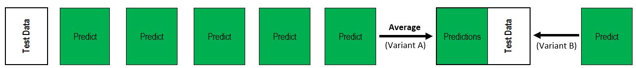
A set of models make predictions, and you average the predictions (or possibly the classification probabilities) to try to decrease the error.
Empirically, a better technique is blended or stacked ensembles:
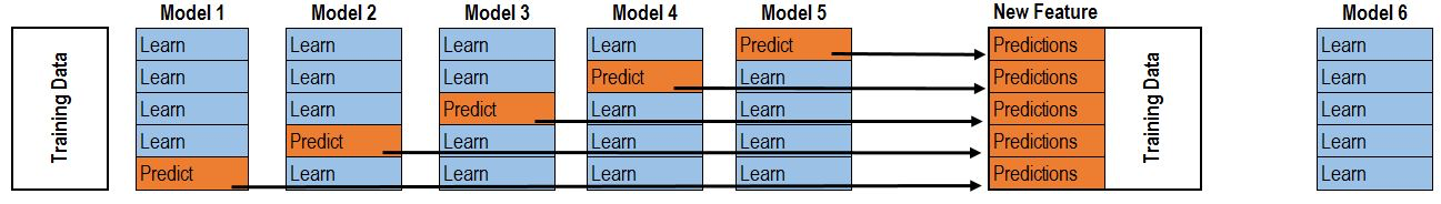
Here, data is split into k-folds. The model is trained on each k-1 fold, and then evaluated on each holdout. Combined, each holdout set recovers the original data set. Then those holdout predictions are now a new feature to build included in an overall ensemble.
The Task
Let’s build an ensemble for the iris dataset, which is a multiclass classification dataset. Other packages such as caretEnsemble do not yet support multiclass ensembles, but leadr provides some tools to handle this situation.
First, let’s build a list of models.
library(purrr)
library(caret)
library(leadr)
folds <- createFolds(iris$Species, k = 5, returnTrain = TRUE)
control <- trainControl(method = 'cv', index = folds, savePredictions = 'final')
mapped_list <- map(
c('rf', 'glmnet'),
~train(
Species ~ .,
data = iris,
method = .,
trControl = control
)
)We explicitly define the cross-validation index, because blending requires that each model is trained on the same set of folds.
We can also specify additional models using caretEnsemble.
library(caretEnsemble)
ensemble_list <- caretList(
  Species ~ .,
  data = iris,
  trControl = control,
  methodList = c('rpart', 'knn')
)
models <- c(mapped_list, ensemble_list)
walk(models, board)
board()
#> # A tibble: 4 x 13
#> rank id dir model metric score public method num group index
#> <dbl> <id> <chr> <chr> <chr> <dbl> <dbl> <chr> <dbl> <dbl> <list>
#> 1 1. 2 models… glmnet Accur… 0.973 NA cv 10. 1. <list…
#> 2 1. 4 models… knn Accur… 0.973 NA cv 10. 1. <list…
#> 3 3. 1 models… rf Accur… 0.953 NA cv 10. 1. <list…
#> 4 4. 3 models… rpart Accur… 0.947 NA cv 10. 1. <list…
#> # ... with 2 more variables: tune <list>, seeds <list>Submodel Selection
We also want to evaluate the models that go into our ensemble. In general, we want to use two different criteria.
First, we want to maximize accuracy, as measured by the 5-fold cross-validation that we build our models on. Second, we want to minimize the prediction correlation. Suppose two sets of model predictions have similar accuracy scores, but are not correlated. This means that each model learned something different about the dataset, and an ensemble could combine those different understandings.
Here are some caret functions to look at those criteria:
results <- resamples(models)
summary(results)
#>
#> Call:
#> summary.resamples(object = results)
#>
#> Models: Model1, Model2, rpart, knn
#> Number of resamples: 5
#>
#> Accuracy
#>             Min.   1st Qu.    Median      Mean   3rd Qu.      Max. NA's
#> Model1 0.8666667 0.9666667 0.9666667 0.9533333 0.9666667 1.0000000    0
#> Model2 0.9333333 0.9666667 0.9666667 0.9733333 1.0000000 1.0000000    0
#> rpart  0.9000000 0.9333333 0.9666667 0.9466667 0.9666667 0.9666667    0
#> knn    0.9000000 0.9666667 1.0000000 0.9733333 1.0000000 1.0000000    0
#>
#> Kappa
#>        Min. 1st Qu. Median Mean 3rd Qu. Max. NA's
#> Model1 0.80    0.95   0.95 0.93    0.95 1.00    0
#> Model2 0.90    0.95   0.95 0.96    1.00 1.00    0
#> rpart  0.85    0.90   0.95 0.92    0.95 0.95    0
#> knn    0.85    0.95   1.00 0.96    1.00 1.00    0

modelCor(results)
#>           Model1    Model2     rpart       knn
#> Model1 1.0000000 0.8669214 0.8846517 0.9355852
#> Model2 0.8669214 1.0000000 0.5345225 0.6416889
#> rpart  0.8846517 0.5345225 1.0000000 0.9861169
#> knn    0.9355852 0.6416889 0.9861169 1.0000000
splom(results)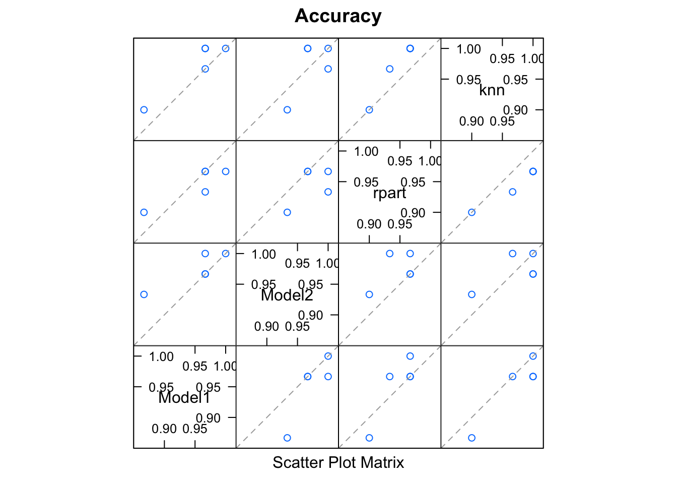
Some of our models are correlated, which is to be expected for a simple data set.
The next step as described in the introductory diagram, is to create a new feature for each model from the out of fold predictions. leadr::oof_grab does this automatically:
blended <- oof_grab(models)
blended
#> # A tibble: 150 x 5
#>    value  value1 value2 value3 Species
#>    <fct>  <fct>  <fct>  <fct>  <fct>
#>  1 setosa setosa setosa setosa setosa
#>  2 setosa setosa setosa setosa setosa
#>  3 setosa setosa setosa setosa setosa
#>  4 setosa setosa setosa setosa setosa
#>  5 setosa setosa setosa setosa setosa
#>  6 setosa setosa setosa setosa setosa
#>  7 setosa setosa setosa setosa setosa
#>  8 setosa setosa setosa setosa setosa
#>  9 setosa setosa setosa setosa setosa
#> 10 setosa setosa setosa setosa setosa
#> # ... with 140 more rows
Now we fit a final ensemble model on the blended data:
ensemble <- train(Species ~ ., data = blended, method = 'rf', trControl = control)
ensemble
#> Random Forest
#>
#> 150 samples
#>   4 predictor
#>   3 classes: 'setosa', 'versicolor', 'virginica'
#>
#> No pre-processing
#> Resampling: Cross-Validated (10 fold)
#> Summary of sample sizes: 120, 120, 120, 120, 120
#> Resampling results across tuning parameters:
#>
#>   mtry  Accuracy  Kappa
#>   2     0.96      0.94
#>   5     0.96      0.94
#>   8     0.96      0.94
#>
#> Accuracy was used to select the optimal model using the largest value.
#> The final value used for the model was mtry = 2.
Then we can add it to our leaderboard and see how it compares to the individual models. We’ll also take advantage of the dir argument of board. Saving this model to a new directory called ensembles allows a natural grouping of the baseline and ensemble models.
board(ensemble, dir = "ensembles")
#> # A tibble: 5 x 13
#>    rank    id dir     model  metric score public method   num group index
#>   <dbl>  <id> <chr>   <chr>  <chr>  <dbl>  <dbl> <chr>  <dbl> <dbl> <list>
#> 1    1.     2 models… glmnet Accur… 0.973     NA cv       10.    1. <list…
#> 2    1.     4 models… knn    Accur… 0.973     NA cv       10.    1. <list…
#> 3    3.     5 ensemb… rf     Accur… 0.960     NA cv       10.    1. <list…
#> 4    4.     1 models… rf     Accur… 0.953     NA cv       10.    1. <list…
#> 5    5.     3 models… rpart  Accur… 0.947     NA cv       10.    1. <list…
#> # ... with 2 more variables: tune <list>, seeds <list>
Conclusions
leadr provides some tools to help build the ensemble, as well as keeping track of the results. We can also use the dir argument of leadr::board to create natural groupings in the leaderboard, such as base models versus ensembles.