Introduction
Tim Mastny
2018-03-08
This vignette will show the basics of the leadr workflow. To see how leadr supports more advanced ensemble model building, check out my Ensembles vignette.
leadr is designed to create one leaderboard per R project per dataset. Currently, the leaderboard works best placed at the project root, with any number of subdirectories to save the models.
Getting Started
library(purrr)
library(tidyverse)
library(caret)
library(leadr)
Let’s build some models. We can easily build a list of models using purrr::map.
We can also purrr the models into our leaderboard. This time we use purrr::walk to update the leaderboard while returning quietly.
walk(models, board)
board()
#> # A tibble: 4 x 13
#>    rank    id dir     model metric  score public method   num group index
#>   <dbl>  <id> <chr>   <chr> <chr>   <dbl>  <dbl> <chr>  <dbl> <dbl> <list>
#> 1    1.     2 models… rf    Accura… 0.955     NA boot     25.    2. <list…
#> 2    2.     4 models… rf    Accura… 0.950     NA boot     25.    4. <list…
#> 3    3.     3 models… rf    Accura… 0.946     NA boot     25.    3. <list…
#> 4    4.     1 models… rf    Accura… 0.942     NA boot     25.    1. <list…
#> # ... with 2 more variables: tune <list>, seeds <list>
By default, board saves the models into a folder at the root of the project called models_one and returns a tibble that provides us with everything we want to know about the model.
The tibble gives us the ranking and metric score, as well as lists like tune, index, and seeds that allow us to exactly recreate the model.
Groups
Of course, fitting four random forest models on the same dataset isn’t very realistic. We’d like to fit a variety of models and compare the accuracy. Let’s use the index column of the leaderboard to fit a new model on the same bootstrap resamples as the first model.
first_id <- which(board()$id == 1)
control <- trainControl(index = board()$index[[first_id]])
model <- train(Species ~ ., data = iris, method = 'glmnet', trControl = control)
board(model)
#> # A tibble: 5 x 13
#>    rank    id dir     model  metric score public method   num group index
#>   <dbl>  <id> <chr>   <chr>  <chr>  <dbl>  <dbl> <chr>  <dbl> <dbl> <list>
#> 1    1.     2 models… rf     Accur… 0.955     NA boot     25.    2. <list…
#> 2    2.     5 models… glmnet Accur… 0.952     NA boot     25.    1. <list…
#> 3    3.     4 models… rf     Accur… 0.950     NA boot     25.    4. <list…
#> 4    4.     3 models… rf     Accur… 0.946     NA boot     25.    3. <list…
#> 5    5.     1 models… rf     Accur… 0.942     NA boot     25.    1. <list…
#> # ... with 2 more variables: tune <list>, seeds <list>
caret has a nice set of functions to compare models trained on the same bootstrap or cross-validation index. To find these comparable models, we can filter on the group column and use leadr::to_list() to convert the filtered leaderboard to a list of models.
From there, we can compare models using the resamples family of caret functions:
results <- resamples(group)
summary(results)
#>
#> Call:
#> summary.resamples(object = results)
#>
#> Models: Model1, Model2
#> Number of resamples: 25
#>
#> Accuracy
#>             Min.   1st Qu.    Median      Mean   3rd Qu.      Max. NA's
#> Model1 0.9107143 0.9433962 0.9473684 0.9516469 0.9655172 1.0000000    0
#> Model2 0.8928571 0.9298246 0.9433962 0.9416994 0.9629630 0.9814815    0
#>
#> Kappa
#>             Min.   1st Qu.    Median      Mean   3rd Qu.      Max. NA's
#> Model1 0.8638794 0.9152452 0.9197047 0.9266939 0.9478886 1.0000000    0
#> Model2 0.8365759 0.8944444 0.9152452 0.9116796 0.9444444 0.9720352    0

modelCor(results)
#>           Model1    Model2
#> Model1 1.0000000 0.6676862
#> Model2 0.6676862 1.0000000
splom(results)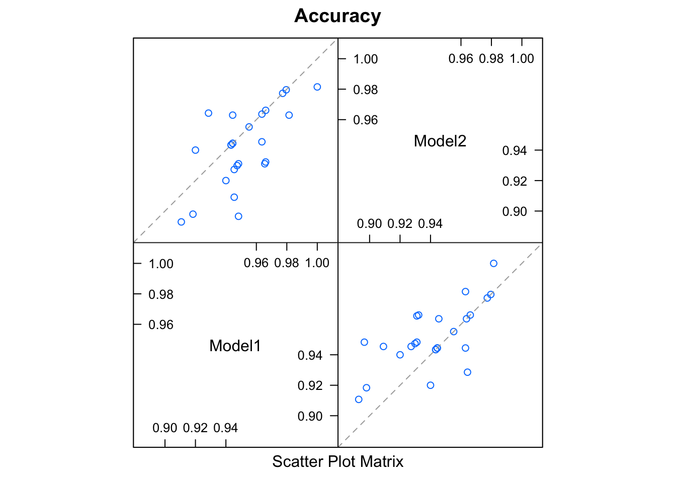
Peaking
leadr also has tools to help you evaluate model ranking as the leaderboard gets big. Let’s add a few more models:
models <- map(
  rep("rf", 20),
  ~train(
    Species ~ .,
    data = iris
  )
)

walk(models, board)
board()
#> # A tibble: 25 x 13
#>     rank    id dir     model metric score public method   num group index
#>    <dbl>  <id> <chr>   <chr> <chr>  <dbl>  <dbl> <chr>  <dbl> <dbl> <list>
#>  1    1.    25 models… rf    Accur… 0.959     NA boot     25.   24. <list…
#>  2    2.    21 models… rf    Accur… 0.959     NA boot     25.   20. <list…
#>  3    3.     6 models… rf    Accur… 0.956     NA boot     25.    5. <list…
#>  4    4.    16 models… rf    Accur… 0.955     NA boot     25.   15. <list…
#>  5    5.     2 models… rf    Accur… 0.955     NA boot     25.    2. <list…
#>  6    6.     9 models… rf    Accur… 0.953     NA boot     25.    8. <list…
#>  7    7.     7 models… rf    Accur… 0.953     NA boot     25.    6. <list…
#>  8    8.    20 models… rf    Accur… 0.953     NA boot     25.   19. <list…
#>  9    9.    17 models… rf    Accur… 0.952     NA boot     25.   16. <list…
#> 10   10.     5 models… glmn… Accur… 0.952     NA boot     25.    1. <list…
#> # ... with 15 more rows, and 2 more variables: tune <list>, seeds <list>
By default the tibble package prints at most 20 rows and only 10 rows for larger tibbles. With leadr::peak, we can peak at the ranking of the first model and those in the surrounding positions:
board() %>%
  peak(1)
#> # A tibble: 10 x 13
#>     rank    id dir     model metric score public method   num group index
#>    <dbl>  <id> <chr>   <chr> <chr>  <dbl>  <dbl> <chr>  <dbl> <dbl> <list>
#>  1   16.    24 models… rf    Accur… 0.950     NA boot     25.   23. <list…
#>  2   17.    19 models… rf    Accur… 0.949     NA boot     25.   18. <list…
#>  3   18.     8 models… rf    Accur… 0.949     NA boot     25.    7. <list…
#>  4   19.    11 models… rf    Accur… 0.946     NA boot     25.   10. <list…
#>  5   20.     3 models… rf    Accur… 0.946     NA boot     25.    3. <list…
#>  6   21.    10 models… rf    Accur… 0.945     NA boot     25.    9. <list…
#>  7   22.    12 models… rf    Accur… 0.944     NA boot     25.   11. <list…
#>  8   23.     1 models… rf    Accur… 0.942     NA boot     25.    1. <list…
#>  9   24.    13 models… rf    Accur… 0.939     NA boot     25.   12. <list…
#> 10   25.    18 models… rf    Accur… 0.938     NA boot     25.   17. <list…
#> # ... with 2 more variables: tune <list>, seeds <list>
We also peak at the last model ran:
board() %>%
peak(at_last())
#> # A tibble: 10 x 13
#> rank id dir model metric score public method num group index
#> <dbl> <id> <chr> <chr> <chr> <dbl> <dbl> <chr> <dbl> <dbl> <list>
#> 1 1. 25 models… rf Accur… 0.959 NA boot 25. 24. <list…
#> 2 2. 21 models… rf Accur… 0.959 NA boot 25. 20. <list…
#> 3 3. 6 models… rf Accur… 0.956 NA boot 25. 5. <list…
#> 4 4. 16 models… rf Accur… 0.955 NA boot 25. 15. <list…
#> 5 5. 2 models… rf Accur… 0.955 NA boot 25. 2. <list…
#> 6 6. 9 models… rf Accur… 0.953 NA boot 25. 8. <list…
#> 7 7. 7 models… rf Accur… 0.953 NA boot 25. 6. <list…
#> 8 8. 20 models… rf Accur… 0.953 NA boot 25. 19. <list…
#> 9 9. 17 models… rf Accur… 0.952 NA boot 25. 16. <list…
#> 10 10. 5 models… glmn… Accur… 0.952 NA boot 25. 1. <list…
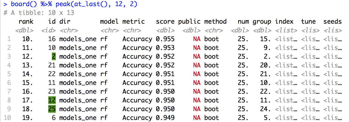
#> # ... with 2 more variables: tune <list>, seeds <list>leadr::peak also takes a variable number of inputs. If we want to compare the last model to the first model, it will return the smallest tibble that contains both. If it is 20 rows or under, it will print the entire tibble.
board() %>%
  peak(at_last(), 1)
#> # A tibble: 23 x 13
#>     rank    id dir     model metric score public method   num group index
#>    <dbl>  <id> <chr>   <chr> <chr>  <dbl>  <dbl> <chr>  <dbl> <dbl> <list>
#>  1    1.    25 models… rf    Accur… 0.959     NA boot     25.   24. <list…
#>  2    2.    21 models… rf    Accur… 0.959     NA boot     25.   20. <list…
#>  3    3.     6 models… rf    Accur… 0.956     NA boot     25.    5. <list…
#>  4    4.    16 models… rf    Accur… 0.955     NA boot     25.   15. <list…
#>  5    5.     2 models… rf    Accur… 0.955     NA boot     25.    2. <list…
#>  6    6.     9 models… rf    Accur… 0.953     NA boot     25.    8. <list…
#>  7    7.     7 models… rf    Accur… 0.953     NA boot     25.    6. <list…
#>  8    8.    20 models… rf    Accur… 0.953     NA boot     25.   19. <list…
#>  9    9.    17 models… rf    Accur… 0.952     NA boot     25.   16. <list…
#> 10   10.     5 models… glmn… Accur… 0.952     NA boot     25.    1. <list…
#> # ... with 13 more rows, and 2 more variables: tune <list>, seeds <list>
Thanks to pillar and crayon, leadr::peak also has special printing when used in a supported console. Here is an example of peak in the RStudio console. Notice that it highlights the peaked models in the console output.